Overview

It’s been more than a year since I started working on my first small scale CAD-like application, which I had to develop from scratch. During that time I managed to accumulate a short list of the most useful 3D geometry formulas and implemented them as algorithms. Some of them are quite simple and straightforward, while others made me search and derive formulas. In this post I will present several basic algorithms that are very likely to be used within any CAD application.

For coding snippets I will be using OpenSceneGraph API. All the algorithms will be presented mathematically first, so you can use any other library or language in order to implement them. In most of the cases we will only be using operators such as multiplication, addition and subtraction of matrices, vectors and scalars.

For quick reference, these are some OpenSceneGraph matrix-vector operators:

• float c = a*b is a dot product between two vectors a and b,
• Vec3 f = a^b is a cross product,
• Vec3 r = v * M is multiplication between a matrix M and vector v,
• Vec3 r = v * s is scaling of vector v by value s.

OpenSceneGraph also offers an osg::Plane class which already contains some useful functions such as plane.intersect(ray) or plane.dotProductNormal(). For more info on the osg::Plane class, refer to the official documentation. The plane class will be useful in some occasions.

Note: The presented code snippets are provided for demonstration purpose and therefore are not necessary robust. It is strongly recommended to check every code snippet before usage in your code against all the corner cases.

Each presented algorithm will have the following format:

• Application example - higher level functions where the algorithm could be applied.
• Mathematical formula derivation.
• Code snippet using OpenSceneGraph API.

The algorithms

Project point on a line (3D or 2D)

Application example: the point on line projection is a very low lever routine. An example of its usage is when we want to calculate the coordinates of intersection line segment of two rectangles in 3D (which is partial case of plane-plane intersection).

We define a line to be given by a parametric (point-and-vector) form:

\[l = P_0 + i\vec{u} \]

Now if we want to project a custom point \( P_i \) onto line \(l\), we can do it by projecting a vector \(\vec{P_0P_1}\) onto the line \(l\). Then if we add the resulting vector to the point \(P_i\), we will obtain the projection result. The final formula is¹:

\[ R = P_i + \frac{ (P_i-P_0) \cdot \vec{u}}{\vec{u}\cdot \vec{u}} \vec{u} \]

Using OpenSceneGraph, we can write the above formula as an algorithm:

/*! \param P0 is the global point on the line.
* \param u is the vector defining the line direction.
* \param Pi is the point to project.
* \return coordinates of the projected point. 
*/
osg::Vec3f projectPointOnLine(const osg::Vec3f& P0, 
                            const osg::Vec3f& u, 
                            const osg::Vec3f& Pi)
{
    return P0 + u * ((Pi-P0)*u)/(u*u);
}

Intersection between two planes (rectangles) in 3D

Application example: Find a line segment of two intersecting rectangles in 3D.

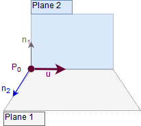
Assuming we are given two planes \(p_1\) and \(p_2\), we want to find a line \(l=P_0+i\vec{u}\) which is an intersection line of the planes (unless the planes are parallel, then no intersection exists). Each plane \(p_i\) (\(i=1,2\)), is given by a point \(C_i\) and a normal vector \(\vec{n_i}\).

Two planes are parallel whenever their normal vectors \(\vec{n_1}\) and \(\vec{n_2}\) are parallel, and this is equivalent to the condition: \(\vec{n_1}\times\vec{n_2}=0\). In the code we could introduce a very small value \(\sigma\) and compare to it in order to avoid division by close-to-zero value, i.e., two planes are parallel when \(\vec{n_1}\times\vec{n_2}<\sigma\).

Two planes intersect in a line which has direction vector \(\vec{u}=\vec{n_1}\times\vec{n_2}\) since \(\vec{u}\) is perpendicular to both \(\vec{n_1}\) and \(\vec{n_2}\), and thus is parallel to both planes as shown on the above figure.

Note: in order to avoid \(|\vec{u}|\) being small, we normalize it making it a unit direction vector.

After the direction vector \(\vec{u}\) is found, we still have to find a specific point \(P_0=(x_0, y_0, z_0)\) on it and which belongs to the both planes. We can do it by finding a solution to the plane equations, but there would be only two equations and the three unknown since the point \(P_0\) can lie anywhere on the line \(l\). For this case we need another constrain to solve for a specific \(P_0\). We will use Direct Linear Equation².

The main idea is to find a non-zero coordinate of \(\vec{u}\) and set the corresponding coordinate of \(P_0\) to 0. Further, we choose the coordinate with the largest absolute value, as this will produce the most robust computations. As an example, suppose \(u_z\neq0\), then we set \(P_0=(x_0,y_0,0\) and it lies on \(l\). Now we have two equations:

\[a_1x_0+b_1y_0+d_1=0 \] \[ a_2x_0+b_2y_0+d_2=0 \]

the solution of which will produce coordinates \(x_0\) and \(y_0\).

Now let’s translate the above math into code using OpenSceneGraph:

/*! A method to calculate intersection line between two planes.
* \param n1 is normal of the first plane,
* \param C1 is arbitrary 3D point on the first plane,
* \param n2 is normal of the second plane,
* \param C2 is arbitrary point on the second plane,
* \param P0 is result point on the intersection line,
* \param u is result directional vector of the intersection line.
* \return 2 if intersection exists and was found.
*/
int getPlanesIntersection(const osg::Vec3f& n1, const osg::Vec3f& C1,
                                    const osg::Vec3f& n2, const osg::Vec3f& C2,
                                    osg::Vec3f& P0, osg::Vec3f& u)
{
    /* cross produc of normals */
    u = n1^n2;

    /* absolute values of u */
    float ax = (u.x() >= 0 ? u.x() : -u.x());
    float ay = (u.y() >= 0 ? u.y() : -u.y());
    float az = (u.z() >= 0 ? u.z() : -u.z());

    /* are two planes parallel? */
    if (std::fabs(ax+ay+az) < EPSILON) { 
        /* normals are near parallel */
        /* are they disjoint or coincide? */
        osg::Vec3f v = C2- C1;
        v.normalize();
        /* coincide */
        if (n1*v == 0) return 1;
        /* disjoint */
        else return 0;
    }

    /* canvases intersect in a line */
    int maxc; // coordinate dimention index
    if (ax > ay) {
        if (ax > az) maxc =  1;
        else maxc = 3;
    }
    else {
        if (ay > az) maxc =  2;
        else maxc = 3;
    }

    /* obtain a point on the intersection line:
     * zero the max coord, and solve for the other two */
    float d1 = -n1*C1; 
    float d2 = -n2*C2; // the constants in the 2 plane equations

    /* result coordinates */
    float xi, yi, zi;
    switch (maxc) {
    case 1:
        xi = 0;
        yi = (d2*n1.z() - d1*n2.z()) /  u.x();
        zi = (d1*n2.y() - d2*n1.y()) /  u.x();
        break;
    case 2:                     // intersect with y=0
        xi = (d1*n2.z() - d2*n1.z()) /  u.y();
        yi = 0;
        zi = (d2*n1.x() - d1*n2.x()) /  u.y();
        break;
    case 3:                     // intersect with z=0
        xi = (d2*n1.y() - d1*n2.y()) /  u.z();
        yi = (d1*n2.x() - d2*n1.x()) /  u.z();
        zi = 0;
    }
    P0 = osg::Vec3f(xi, yi, zi);
    return 2;
}

Intersection between plane and a ray/line

Application example: the most common example is ray casting at a virtual plane, i.e., when we want to get an intersection of the ray cast from mouse coordinates with certain plane on the scene, e.g., drawing a line on a plane.

A plane can be described by a set of points for which

\[(P-C)\vec{n}=0\]

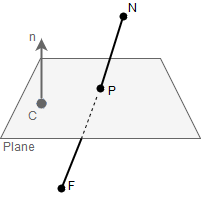
Where \(\vec{n}\) is a normal vector to the plane, and \(C\) is an arbitrary point on the plane.

The line segment, or a ray, or a line is represented by two points in 3D - \(N\) and \(F\) (like if we are talking about near and far points). Our task is to find an intersection between the line segment \(NF\) and the plane.

Generally speaking, if we deal with a line (not line segment which is restricted by two points, or a ray which is restricted by one point), it will be either parallel to any plane in 3D, or intersect it at some point. We can check whether the line and plane are parallel by testing if \(\vec{n}\cdot\vec{FN}=0\), which means that the line direction vector \(\vec{FN}\) is perpendicular to the plane normal \(\vec{n}\). If this is true, there can be no intersection found since the line is parallel to the plane.

If the line and the plane are not parallel, they have an intersection point \(P\) which can be found as²:

\[x = \frac{(C-N)\cdot\vec{n}}{\vec{FN}\cdot\vec{n}} \] \[P = \vec{FN}x + N\]

When we convert the above formulas into OpenSceneGraph code, we can take advantage of the osg::Plane class and its implemented methods that check whether a specific ray intersects a plane, or located above/below the plane. Of course, if we want to calculate the intersection between a line and a plane, then that part must be omitted.

/*! A method to calculate an intersection between a plane and line or ray. 
* \param plane is the input plane,
* \param center is the arbitrary point that belongs to the plane,
* \param nearPoint is one of the two points that belongs to the input line/ray,
* \param farPoint is the second point that belongs to the input line/ray,
* \param P is the result point,
* \param isLine indicated whether we deal with line (true) or line segment (false) intersections.
* \return true if the intersection was found, false - otherwise. 
*/
bool getRayPlaneIntersection(const osg::Plane &plane, const osg::Vec3f &center, 
                             const osg::Vec3f &nearPoint, const osg::Vec3f &farPoint, 
                             osg::Vec3f &P, 
                             bool isLine)
{
    if (!plane.valid())
        return false;

    // if it is ray segment, check whether it intersects at all
    if (!isLine) {
        std::vector<osg::Vec3f> ray(2);
        ray[0] = nearPoint;
        ray[1] = farPoint;
        if (plane.intersect(ray)) { // 1 or -1 means no intersection
            std::cout << "Ray lies above or below the plane.\n";
            return false;
        }
    }

    osg::Vec3f dir = farPoint-nearPoint;
    // check if line is parallel
    if (!plane.dotProductNormal(dir)){
        std::cout << "The line is parallel to the plane.\n";
        return false;
    }

    // check if plane contains the line
    if (! plane.dotProductNormal(center-nearPoint)){
        std::cout << "Plane contains the line.\n";
        return false;
    }

    double x = plane.dotProductNormal(center-nearPoint) / plane.dotProductNormal(dir);
    P = dir * x + nearPoint;

    return true;
}

Skew lines geometry: shortest distance and projection of one skew line onto another

Application example: Dragging of a rectangle along its normal by using a ray cast from mouse position. The 3D ray cast and the rectangle’s normal are skew lines in 3d, and the new position of the rectangle is estimated as a 3D projection of one skew line onto another.

At one of my previous tutorials I already had referred to the geometry of skew lines when demonstrating how to improve line intersector. That time we demonstrated how to calculate the shortest distance between two skew lines. This algorithm is an extension of the shortest distance algorithm since it will allow calculation of the projection coordinates.

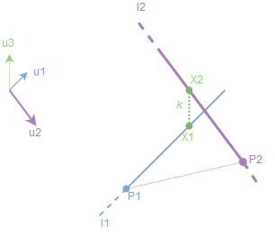
Assuming we are given a line/ray (e.g., result of the ray casting algorithm) \(l_1\) with a point \(P_1\). Another line is given by a line \(l_2\) and corresponding point \(P_2\).

Now we want to perform a projection of the line \(l_2\) onto \(l_1\), i.e., we want to calculate 3D coordinates of the point \(X_1\) (or inversely of \(X_2\), if needed).

Let \(\vec{d} = P_1 - P_2\) is the direction vector from \(R_1\) to \(X_1\). Let \(\vec{u_1}\) and \(\vec{u_2}\) be unit direction vectors for the given line segments. Then we can obtain an orthogonal to both \(l_1\) and \(l_2\): it can be found by cross product between \(\vec{u_1}\) and \(\vec{u_2}\), i.e., \(\vec{u_3} = \vec{u_1}\times \vec{u_2}\). Now if we project \(\vec{d}\) onto \(\vec{u_3}\) we will obtain a scalar result which is the shortest distance between the two skew lines³:

\[d = \frac{\vec{d}\cdot(\vec{u_1}\times\vec{u_2})}{|\vec{u_1} \times \vec{u2} |}\]

Note: since the skew lines are not parallel, \(\vec{u_1}\times\vec{u_2}\neq 0\).

We want to calculate the position of \(X_1\) and \(X_2\) - the closest points on the lines. Let \(\vec{k}=\vec{X_1X_2}\), and let \(r_i\) be the unique numbers such that \(X_i = P_i + r_i\vec{u_i}\). Given \(\vec{k}\) is orthogonal to both lines, taking the dot product of \(\vec{u_1}\cdot\vec{u_2}\) yields the system of linear equations³ (derivation omitted):

\[\vec{u_1}\cdot\vec{u_1}r_1 - \vec{u_1}\cdot\vec{u2}r_2 - \vec{u_1}\cdot\vec{d} = 0\] \[\vec{u_1}\cdot\vec{u_2}r_1 - \vec{u_2}\cdot\vec{u2}r_2 - \vec{u_2}\cdot\vec{d} = 0\]

for \(r_1\) and \(r_2\). From the above equations we can obtain \(X_i\). E.g., the derivation steps for the point \(X_1\) will be:

1. Let \(a_1 = \vec{u_1}\cdot\vec{u_1}\), \(b_1 = \vec{u_1}\cdot\vec{u_2}\) and \(c_1 = \vec{u_1}\cdot\vec{d}\).
2. Let \(a_2 = \vec{u_1}\cdot\vec{u_2}\), \(b_2 = \vec{u_2}\cdot\vec{u_2}\) and \(c_2 = \vec{u_2}\cdot\vec{d}\).
3. Calculate \(r_1 = \frac{c_2-\dfrac{b_2c_1}{b_1}}{a_2-\dfrac{b_2a_1}{b_1}}\).
4. Calculate \(X_1 = P_1 + r_1\vec{u_1}\).

Given the above formula, it is straightforward to implement both algorithms using OpenSceneGraph.

The shortest distance code:

/*! An algorithm to calculate the shortest distance between two skew lines. 
* \param P1 is the first point of the first line,
* \param P12 is the second point on the first line,
* \param P2 is the first point on the second line,
* \param P22 is the second point on the second line.
* \return the shortest distance
*/
double getSkewLinesDistance(const osg::Vec3d &P1, const osg::Vec3d &P12, 
                            const osg::Vec3d &P2, const osg::Vec3d &P22)
{
    osg::Vec3d u1 = P12-P1;
    osg::Vec3d u2 = P22-P2;
    osg::Vec3d u3 = u1^u2;
    if (u3.length() == 0) return 1;
    u3.normalize();
    osg::Vec3d dir = P1 - P2;
    return std::fabs((dir*u3)); // u3 is already normalized
}

The projection algorithm:

/*! A method to project one skew line onto another. 
* \param P1 is a first point that belonds to first skew line,
* \param P12 is the second point that belongs to first skew line,
* \param P2 is the first point that belongs to second skew line,
* \param P22 is the second point that belongs to second skew line,
* \param X1 is the result projection point of line P2P22 onto line P1P12. 
* \return true if such point exists, false - otherwise.
*/
bool getSkewLinesProjection(const osg::Vec3f &P1, const osg::Vec3f &P12, 
                            const osg::Vec3f &P2, const osg::Vec3f &P22, 
                            osg::Vec3f &X1)
{
    osg::Vec3f d = P2 - P1;
    osg::Vec3f u1 = P12-P1;
    u1.normalize();
    osg::Vec3f u2 = P22 - P2;
    u2.normalize();
    osg::Vec3f u3 = u1^u2;

    double EPSILON = 0.00001;
    if (std::fabs(u3.x())<=EPSILON && 
        std::fabs(u3.y())<=EPSILON && 
        std::fabs(u3.z())<=EPSILON){
        std::cout << "The rays are almost parallel.\n";
        return false;
    }

    // X1 and X2 are the closest points on lines
    // we want to find X1 (lies on u1)
    // solving the linear equation in r1 and r2: Xi = Pi + ri*ui
    // we are only interested in X1 so we only solve for r1.
    float a1 = u1*u1, b1 = u1*u2, c1 = u1*d;
    float a2 = u1*u2, b2 = u2*u2, c2 = u2*d;
    if (!(std::fabs(b1) > EPSILON)){
        std::cout << "Denominator is close to zero.\n";
        return false;
    }
    if (!(a2!=-1 && a2!=1)){
        std::cout << "Lines are parallel.\n";
        return false;
    }

    double r1 = (c2 - b2*c1/b1)/(a2-b2*a1/b1);
    X1 = P1 + u1*r1;

    return true;
}

Intersection between two lines in 3D using skew lines geometry

In 3D two lines are very unlikely to intersect. However, we can use skew lines geometry algorithms of the shortest distance and of the projection points calculation in order to easily extract a 3D intersection point of two lines in 3D. This algorithm could also be useful when we want to extract an approximate intersection point, i.e., lines do not strictly intersect, but within an Euclidean distance of very small value, which could occur due to computations. For this purpose, we can separate the algorithm into two parts: first, if there is a precise intersection, and second, if the intersection is approximate.

The steps of the algorithm are as follows:

1. Treat the two lines as skew lines.
2. Calculate the shortest distance between the two skew lines.
3. If the distance is zero, the lines intersect precisely; find the intersection using dot and cross products.
4. If the intersection is not precise, extract the intersection point as average between two projections of both of the skew lines.

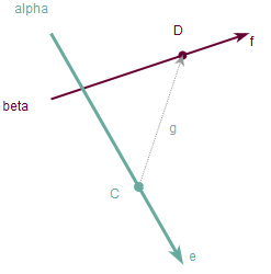
As mentioned above, the formula for the precise intersection can be found using dot and cross product of vectors⁴. Let \(\alpha\) and \(\beta\) be two 3D lines which are given by points \(C\) and \(D\) and direction vectors \(\vec{e}\) and \(\vec{f}\) correspondingly.

Let \(\vec{g} = \vec{CD}\) be a direction vector from point \(D\) to point \(C\).

Note: if either \(\lvert \vec{f}\times\vec{g}\rvert\) or \(\lvert\vec{f}\times\vec{e}\rvert\) is zero, then the lines are parallel and have no intersection point.

In order to calculate the final intersection point \(P\), we have to derive scaling factor \(s\) which would equate \(P=C\pm s\vec{e}\), where the sign depedens on the directions of the vectors \(\vec{f}\) and \(\vec{e}\). The scaling factor iteself can be derived using length of cross products: \(s=\frac{\lvert\vec{f}\times\vec{g}\rvert}{\lvert\vec{f}\times\vec{e}\rvert}\). Using all together results in:

\[P=C\pm \frac{\lvert \vec{f}\times\vec{g} \rvert}{\lvert \vec{f}\times\vec{e} \rvert}\vec{e}\]

where the sign is defined: if \(\vec{f}\times\vec{g}\) and \(\vec{f}\times\vec{e}\) point in the same direction, the sign is \(+\), otherwise it is \(-\).

Now we can provide OpenSceneGraph-based implementation for two lines intersection in 3D:

/*! An algorithm to calculate an (approximate) intersection of two lines in 3D.
* \param La1 is the first point on the first line,
* \param La2 is the second point on the first line,
* \param Lb1 is the first point on the second line,
* \param Lb2 is the second point on the second line,
* \param intersection is the result intersection, of it can be found.
* \return true if the intersection can be found, false - otherwise.
*/
bool getLinesIntersection(const osg::Vec3f &La1, const osg::Vec3f &La2, 
                            const osg::Vec3f &Lb1, const osg::Vec3f &Lb2, 
                            osg::Vec3f &intersection)
{
    // first check if lines have an exact intersection point
    // do it by checking if the shortest distance is exactly 0
    float distance = getSkewLinesDistance(La1, La2, Lb1, Lb2);
    if (distance == 0.f){
        std::cout << "3d lines have exact intersection point\n";
        osg::Vec3f C = La2;
        osg::Vec3f D = Lb2;
        osg::Vec3f e = La1-La2;
        osg::Vec3f f = Lb1-Lb2;
        osg::Vec3f g = D-C;
        if ((f^g).length()==0 || (f^e).length()==0){
            std::cout << "Lines have no intersection, are they parallel?\n";
            return false;
        }

        osg::Vec3f fgn = f^g; 
        fgn.normalize();
        
        osg::Vec3f fen = f^e; 
        fen.normalize();
        
        int di = -1;
        if (fgn == fen) // same direction?
            di *= -1;

        intersection = C + e*di*( (f^g).length() / (f^e).length() );
        return true;
    }

    // try to calculate the approximate intersection point
    osg::Vec3f X1, X2;
    bool firstIsDone = getSkewLinesProjection(La1, La2, Lb1, Lb2, X1);
    bool secondIsDone = getSkewLinesProjection(Lb1, Lb2, La1, La2, X2);
    
    if (!firstIsDone || !secondIsDone){
        std::cout << "Could not obtain projection point.\n";
        return false;
    }

    intersection = (X1 + X2)/2.f;
    return true;
}

Afterword

Currently I’m trying to figure out what could be a small demo program that would demonstrate the usage of all the presented algorithms. In the future I might link this page to the coded demo, so stay tuned! Meanwhile, I was wondering if there could be any other 3D geometry algorithms to add to the list. So if you have ideas, do not hesitate to let me know in the comment section or by contacting me directly. It is always great to be able to improve the posts from user feedback.